From measurement to analysis
EasyDiffraction compares a crystallographic model with diffraction measurements. Understanding where that comparison begins helps you choose suitable inputs and recognise what a fit can establish.
Acquisition, reduction and analysis
Acquisition
Record the detector response while the sample scatters the incident beam. This example uses a two-dimensional detector.


Reduction
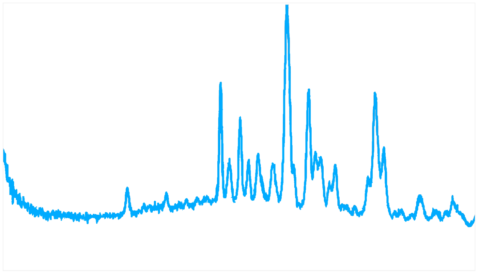
Apply the relevant corrections and turn detector measurements into observations with uncertainties. For powder diffraction, these are often a one-dimensional intensity profile.
Analysis
Compare a calculated pattern with the observations, fit the model and inspect the result. EasyDiffraction focuses on this stage.
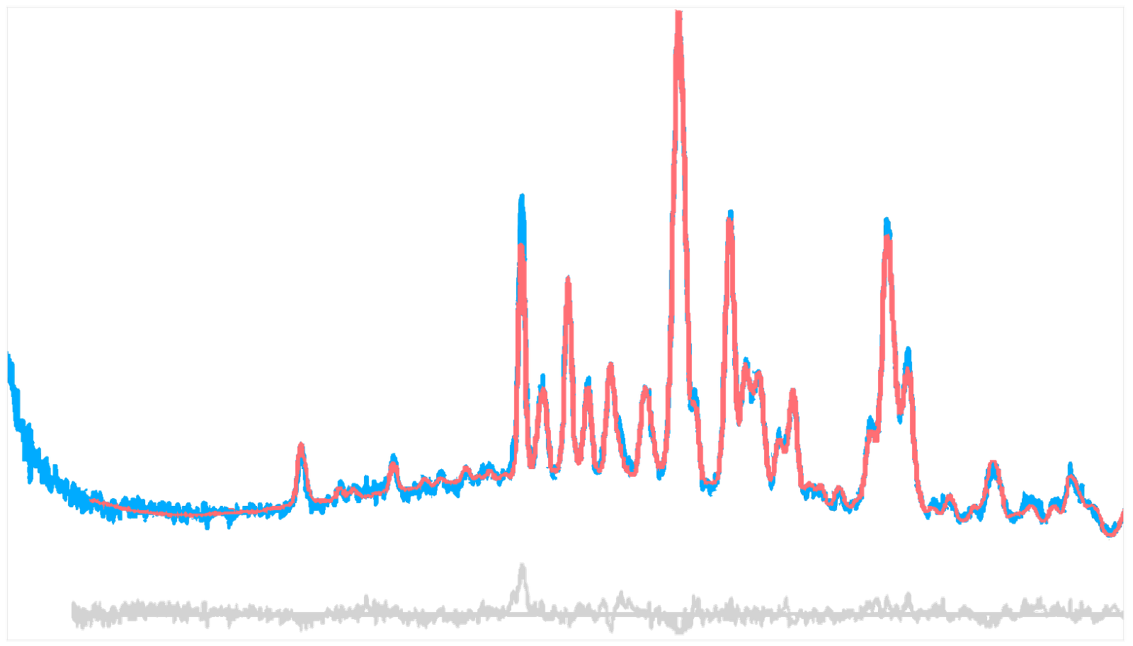
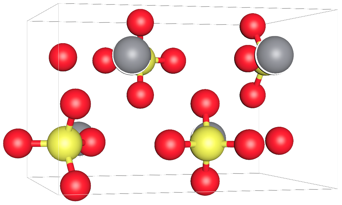
Illustration credits
These illustrations are reused from the earlier EasyDiffraction concept guide. Its detector and diffraction example is credited to Bish et al., Science (2013). They illustrate the processing stages; the tutorials use their own measured examples.
Keep the reduction history and experimental context with the project: they affect how uncertainties and agreement factors should be interpreted.
A model of the sample and the experiment
The calculated intensity depends on more than atom positions. EasyDiffraction separates the model into two connected parts:
A disagreement between measured and calculated patterns can therefore have several causes. A peak-position error may come from the cell or calibration; a broad mismatch underneath peaks may come from the background; an intensity mismatch can involve the structure as well as experiment settings.
Calculation and fitting
A calculation predicts the diffraction pattern from the current structure and experiment. It does not need measured intensities. Use it to inspect peak positions and the influence of the model before fitting.
A fit needs observations to compare against. A least-squares fit reduces the weighted difference between observations and calculations: it changes the parameters marked as free, while fixed parameters still contribute to the calculated pattern. The starting model, free-parameter set, constraints, excluded regions and minimizer conditions all influence the result.
Start from a physically meaningful model. Inspect the initial pattern, allow parameters to vary deliberately, and review the result after each meaningful change. Adding more free parameters may reduce a residual without making the model more informative.
Least squares and Bayesian analysis
Both compare a model with observations, but summarise parameter uncertainty differently.
| Approach | What it reports |
|---|---|
| Least squares | A best-fit parameter set and, when the covariance can be estimated, standard uncertainties and correlations |
| Bayesian sampling | A posterior distribution combining a likelihood with prior information, from which credible intervals and correlations can be summarised |
The fitting instructions in this documentation use least squares. Its objective and covariance conventions explain the reported uncertainties. Bayesian sampling is a separate workflow; the older library's sampler choices should not be assumed to be available in this application.
Interpreting the result
Convergence describes how the optimisation ended. It does not by itself establish that the sample model is correct or that all uncertainty sources have been captured.
Inspect the observed and calculated pattern, the residual, parameter uncertainties and correlations, and the physical plausibility of the result. Fit quality explains these checks in more detail.
The same ideas in every interface
The app makes these relationships visible. Python lets you express them in a script or notebook. The Command line runs the analysis already declared by a saved project. All use the same project model.